Notes on the Bernoulli distribution

Bernoulli distribution describes an outcome of a single experiment with two possible outcomes (success or failure): \(X=1\) if an experiment was successfull, \(X=0\) if it was not.

Parameter: \(p\) – probability of a success.

Values: \(\{0,1\}.\)

Probability mass function: \[ P(X=1)=p, \ P(X=0)=1-p. \]

Moment generating function: \[ M(t)=1-p+pe^t \]

Proof

\[ M(t)=Ee^{tX}=e^t\cdot P(X=1)+e^0\cdot P(X=0)=pe^t+1-p \]

All moments: \[ EX^n=p, \ n\geq 1. \]

Proof

Observe that \(X^n=X,\) for \(n\geq 1.\) Further, \[ EX=1\cdot P(X=1)+0\cdot P(X=0)=p+0=p \]

Expectation: \(EX=p\)

Variance: \(V(X)=p(1-p)\)

#Bernoulli # Statistics # Probability # Elementary

Areas swept up by Spirals

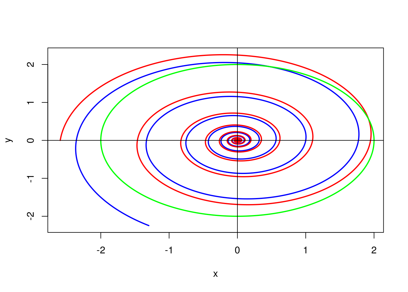
A friend of mine and I were re-visiting Euler’s identity: \(e^{ \pm i\theta } = \cos \theta \pm i\sin \theta\) and we started looking at spirals of the form: \((e^z)^n = [r (\cos \theta \pm i\sin \theta)]^n\) where \(\theta\) and \(r\) are fixed while n varies from \((-\infty, \infty)\)

#swept # Areas # Spirals

Notes on the Binomial distribution

Binomial distribution describes the number of successes in a series of \(n\) independent identical experiments: \(X=k\) if exactly \(k\) experiments out of \(n\) were successfull, while others were not.

Parameters: \(n\) – number of experiments, \(p\) – probability of a success in a single experiment.

Values: \(\{0,1,2,\ldots,n\}.\)

Probability mass function: \[ P(X=k)={n\choose k}p^k(1-p)^{n-k}, \ k=0,1,2,\ldots,n. \]

Derivation

Let \(\xi_k,\) \(k=1,2,\ldots,n,\) be the result of \(k\)-th experiment, i.e. \(\xi_k=1\) if \(k\)-th experiment was successfull, and \(\xi_k=0\) otherwise. Then \[ X=\xi_1+\xi_2+\ldots+\xi_n, \] By assumption, \(\xi_1,\ldots,\xi_n\) are independent and each has a Bernoulli distribution with parameter \(p.\) Event \(\{X=k\}\) means that exactly \(k\) variables of \(\xi_1\ldots,\xi_n\) equal to \(1\) and others are equal to \(0.\) There are \({n\choose k}\) possibilities to choose variables that are equal to \(1.\) Each of them is \(1\) with probability \(p,\) other \(n-k\) variables are \(0\) each with probability \(1-p.\)

Moment generating function: \[ M(t)=(1-p+pe^t)^n \]

Proof

\[ M(t)=Ee^{t(\xi_1+\ldots+\xi_n)}= \] using independence \[ =Ee^{t\xi_1}Ee^{t\xi_2}\ldots Ee^{t\xi_n}=(pe^t+1-p)^n \]

Expectation: \(EX=np\)

Variance: \(V(X)=np(1-p)\)

Derivation

Expectation is the first derivative \(M'(0).\) We have \[ M'(t)=n(pe^t+1-p)^{n-1}pe^t, \ EX=M'(0)=np. \] Second moment is the second derivative \(M''(0).\) We have \[ M''(t)=n(n-1)(pe^t+1-p)^{n-1}p^2e^{2t}+n(pe^t+1-p)^{n-1}pe^t, \] \[ EX^2=M''(0)=n(n-1)p^2+np. \] Variance is \[ V(X)=EX^2-(EX)^2=n(n-1)p^2+np-n^2p^2=np(1-p) \]

#Binomial # Statistics # Probability # Elementary

Notes on the Geometric distribution

Consider simple experiment with two possible outcomes: success or failure. Geometric distribution describes the number of successes in a sequence of independent experiments performed until the first failed one. Formally, if \(\xi_1,\xi_2,\ldots\) are results of experiments (that is all \(\xi\) are independent and have Bernoulli distribution), then the geometric random variables is \[ X=\min\{n\geq 0:\xi_{n+1}=0\}. \] (There are other modifications of a geometric distribution, for example when the first fail is also counted).

Parameters: \(p\) – probability of a success in a single experiment.

Values: \(\{0,1,2,\ldots\}.\)

Probability mass function: \[ P(X=k)=p^k(1-p), \ k\geq 0. \]

Derivation

The event \(X=k\) means that first \(k\) experiments were successfull, and \((k+1)-\)st was not: \[ P(X=k)=P(\xi_1=1,\ldots,\xi_{k}=1,\xi_{k+1}=0)= \] by independence \[ =P(\xi_1=1)\ldots P(\xi_{k}=1)P(\xi_{k+1}=0)=p^{k}(1-p). \]

Moment generating function: \[ M(t)=\frac{(1-p)e^t}{1-pe^t}, \ t< \ln\frac{1}{p} \]

Proof

\[ M(t)=Ee^{tX}= \] using probability mass function \[ =\sum^\infty_{k=0} e^{tk}p^{k}(1-p)=(1-p)\sum^\infty_{k=0} (pe^t)^{k}= \] the sum of a geometric progression with a multiple \(pe^t<1\) (condition on \(t!\)) \[ =\frac{1-p}{1-pe^t} \]

Expectation: \(EX=\frac{p}{1-p}\)

Variance: \(V(X)=\frac{p}{(1-p)^2}\)

Derivation

Expectation is the first derivative \(M'(0).\) We have \[ M'(t)=\frac{(1-p)pe^t}{(1-pe^t)^2} \] \[ EX=\frac{p}{1-p} \] Second moment is the second derivative \(M''(0).\) We have \[ M''(t)=\frac{(1-p)pe^t}{(1-pe^t)^2}+\frac{2(1-p)p^2e^{2t}}{(1-pe^t)^3} \] \[ EX^2=\frac{p}{1-p}+\frac{2p^2}{(1-p)^2} \] Variance is \[ V(X)=\frac{p}{1-p}+\frac{p^2}{(1-p)^2}=\frac{p}{(1-p)^2} \]

#Geometric # Statistics # Probability # Elementary

Notes on the Hypergeometric distribution

In contrast to binomial distribution where the probability of a success is the same for each experiment, the hypergeometric distribution describes situation when the probability of success decreases after each success (and increases after each failure). Each experiment is modelled by an urn containing \(N\) balls, \(K\) of them being ``lucky’’ (and \(N-K\) unlucky). \(n\) draws are performed from an urn and the hypergeometric random variable \(X\) is the numebr of lucky balls drawn. So, each lcuky ball decreases the probability to pick a lucky ball in the next draw. One more point of view is that the hypergeometric distribution models draws without replacement, while binomial models draws with replacement (to keep the probability of picking a lucky ball constant we return the drawn ball back to the urn).

Parameters: \(N\) – number of balls in the urn, \(K\) – number of lucky balls in the urn, \(n\) – number of draws, \(0\leq n\leq N,\) \(0\leq K\leq N.\)

Values: \(\{0,1,2,\ldots,n\}\) (in fact values with nonzero probabilities are \(k\in[\max(0,n-N+K),\min(n,K)]\))

Probability mass function: \[ P(X=k)=\frac{{K\choose k}{N-K\choose n-k}}{{N\choose n}}, \ k=0,1,2,\ldots,n. \] (we agree that \({K\choose k}=0\) for \(k>K\)).

{} There are \({N\choose n}\) possibilities to draw \(n\) balls from an urn containing \(N\) balls. We are interested in draws that contain exactly \(k\) lucky balls. So, satisfactory outcomes are draws that contain \(k\) lucky and \(n-k\) unlucky balls. There are \({K\choose k}{N-K\choose n-k}\) possibilities to perform such draw.

Moment generating function does not have a simple representation: \[ M(t)=\sum^{n}_{k=0}e^{tk}\frac{{K\choose k}{N-K\choose n-k}}{{N\choose n}} \]

Expectation: \(EX=n\frac{K}{N}\)

Variance: \(V(X)=\frac{nK(N-k)(N-n)}{N^2(N-1)}\)

Derivation

We find expectation as a sum over all possible values of \(X:\) \[ EX=\sum^n_{k=0}k \frac{{K\choose k}{N-K\choose n-k}}{{N\choose n}}= \] the summand with \(k=0\) is zero \[ =\frac{1}{{N\choose n}}\sum^n_{k=1}k {K\choose k}{N-K\choose n-k}= \] use the identity \(k{K\choose k}=K{K-1 \choose k-1}\) \[ =\frac{K}{{N\choose n}}\sum^n_{k=1} {K-1 \choose k-1 }{(N-1)-(K-1)\choose (n-1)-(k-1)}= \] change summation variable to \(k-1\) \[ =\frac{K}{{N\choose n}}\sum^{n-1}_{k=0} {K-1 \choose k }{(N-1)-(K-1)\choose (n-1)-k}= \] represent the sum as a sum of all probabilities for hypergeometric distribution with parameters \(N-1,K-1,n-1\) (which is 1) \[ =\frac{K{N-1\choose n-1}}{{N\choose n}}\sum^{n-1}_{k=0} \frac{{K-1 \choose k }{(N-1)-(K-1)\choose (n-1)-k}}{{N-1\choose n-1}}=\frac{K{N-1\choose n-1}}{{N\choose n}}=n\frac{K}{N} \]

Similarly we find \(EX(X-1):\) \[ EX(X-1)=\sum^n_{k=0} k(k-1)\frac{{K\choose k}{N-K\choose n-k}}{{N\choose n}}= \] \[ =\frac{1}{{N\choose n}}\sum^n_{k=2}k(k-1) {K\choose k}{N-K\choose n-k}= \] use the identity \(k(k-1){K\choose k}=K(K-1){K-2 \choose k-2}\) \[ =\frac{K(K-1)}{{N\choose n}}\sum^{n-2}_{k=0} {K-2 \choose k }{(N-2)-(K-2)\choose (n-2)-k}= \] \[ =\frac{K(K-1){N-2\choose n-2}}{{N\choose n}}=n(n-1)\frac{K(K-1)}{N(N-1)} \]

Variance is \[ V(X)=EX^2-(EX)^2=EX(X-1)+EX-(EX)^2=\] \[ =n(n-1)\frac{K(K-1)}{N(N-1)}+n\frac{K}{N}-n^2\frac{K^2}{N^2}= \] \[ =\frac{nKN^2-n^2KN-nK^2N+n^2K^2}{N^2(N-1)}=\frac{nK(N-k)(N-n)}{N^2(N-1)} \]

#Hypergeometric # Statistics # Probability # Elementary

Notes on the Multinomial distribution

A multidimensional generalization of a binomial distribution. Assume that in each experiment there are \(k\) possible outcomes (enumerated by \(1,2,\ldots,k\)). Probabilities of these outcomes are \(p_1,p_2,\ldots,p_k,\) so that \[ p_1,\ldots,p_k\geq 0, \ p_1+\ldots+p_k=1. \] Multinomial distribution describeds the number of outcomes of each type in \(n\) independent repetitions of the experiment:

\((X_1,\ldots,X_k)=(m_1,\ldots,m_k)\) if exactly \(m_1\) experiments resulted in the outcome \(1,\) exactly \(m_2\) experiments resulted in the outcome \(2,\ldots,\) exactly \(m_k\) experiments resulted in the outcome \(k.\)

Parameters: \(n\) – number of experiments, \(k\) – number of outcomes in each experiment, \((p_1,\ldots,p_k)\) – probability distribution of an outcome in each experiment.

Values: all sequences \((m_1,\ldots,m_k)\) of non-negative integers that sum up to \(n\) (there are \({n\choose n+k-1}\) such sequences).

Probability mass function: \[ P(X_1=m_1,\ldots,X_k=m_k)=\frac{n!}{m_1!\ldots m_k!}p^{m_1}_{1}\ldots p^{m_k}_k. \]

Derivation

Let \(\xi_l,\) \(l=1,2,\ldots,n,\) be the result of \(l\)-th experiment, \(\xi_l\in\{1,2,\ldots,k\}.\) The event \[ \{X_1=m_1,\ldots,X_k=m_k\} \] means that exactly \(m_1\) variables \(\xi_l=1,\) exactly \(m_2\) variables \(\xi_l=2,\) \(\ldots,\) exactly \(m_k\) variables \(\xi_l=k.\) When variables \(\xi_1,\ldots,\xi_l\) are already grouped according to their values, the probability becomes \(p^{m_1}_1\ldots p^{m_k}_k.\) The number of partitions of \(n\) elements into \(k\) groups by \(m_1,m_2,\ldots,m_k\) elements is \(\frac{n!}{m_1!\ldots m_k!}\).

Moment generating function: \[ M(t_1,\ldots,t_k)=Ee^{t_1X_1+\ldots+t_kX_k}=(p_1e^{t_1}+\ldots+p_k e^{t_k})^n \]

Proof

\[ M(t_1,\ldots,t_k)=Ee^{t_1X_1+\ldots+t_kX_k}= \] using probability mass function \[ =\sum_{m_1+\ldots+m_k=n}\frac{n!}{m_1!\ldots m_k!}p^{m_1}_1\ldots p^{m_k}_k e^{t_1m_1+\ldots +t_km_k}= \] \[ =\sum_{m_1+\ldots+m_k=n}\frac{n!}{m_1!\ldots m_k!}(p_1e^{t_1})^{m_1}\ldots (p_ke^{t_k})^{m_k}= \] by multinomial formula \[ =(p_1 e^{t_1}+\ldots+p_k e^{t_k})^n \]

Expectation: \(EX_j=np_j,\) \(1\leq j\leq k.\)

Variance: \(V(X_j)=np_j(1-p_j),\) \(1\leq j\leq k\)

Covariance: \(cov(X_i,X_j)=-np_ip_j,\) \(1\leq i<j\leq k.\)

Derivation

The moment generating function of a single variable \(X_j\) is obtained from \(M(t_1,\ldots,t_k)\) by letting \(t_i=0,\) \(i\ne j.\) That is \[ Ee^{t_jX_j}=M(0,\ldots,0,t_j,0,\ldots,0)=(p_1+\ldots+p_{j-1}+p_j e^{t_j}+p_{j+1}+\ldots+p_k)^n= \] using that \(p_1+\ldots+p_k=1\) \[ =(1-p_j+p_je^{t_j})^n \] This is exactly the moment generating function of a binomial distribution with parameters \(n,p_j:\) \[ X_j\sim Binomial(n,p_j) \] In particular \[ EX_j=np_j, \ V(X_j)=np_j(1-p_j). \] To compute expectation of the product \(EX_iX_j,\) \(i\ne j,\) we take second mixed derivative of \(M\) at point zero: \[ \frac{\partial M}{\partial t_i}=np_ie^{t_i}(p_1 e^{t_1}+\ldots+p_k e^{t_k})^n \] \[ \frac{\partial^2 M}{\partial t_i\partial t_j}=n(n-1)p_ip_je^{t_i+t_j}(p_1 e^{t_1}+\ldots+p_k e^{t_k})^{n-2} \] Put \(t_1=\ldots=t_k=0\) and get \[ E X_iX_j=n(n-1)p_ip_j \] So, the covariance \[ cov(X_i,X_j)=EX_iX_j-EX_iEX_j= \] \[ =n(n-1)p_ip_j-n^2p_ip_j=-np_ip_j. \]

#Multinomial #Statistics #Probability

Notes on the Negative binomial distribution

A generalization of a geometric distribution. Negative binomial distribution describes the number of successes in a sequence of independent experiments performed until the \(r-\)th failure. Formally, let \(\xi_1,\xi_2,\ldots\) are results of experiments (that is all \(\xi\) are independent and have Bernoulli distribution). \(S_n=\xi_1+\ldots+\xi_n\) is the cumulative sum of \(\xi'\)s that represents the number of successes. The fact that there were \(r\) failures can be written as \(S_n=n-r.\) So, the negative binomial random variables is \[ X=S_\tau, \tau=\min\{n\geq 1:S_n=n-r\} \] (here \(\tau\) is the number of the last experiment, when \(r\)-th failure occured).

Parameters: \(r\) – number of failures after which we stop performing experiments, \(p\) – probability of a success in a single experiment.

Values: \(\{0,1,2,\ldots\}.\)

Probability mass function: \[ P(X=k)={k+r-1\choose k}p^{k}(1-p)^r, \ k\geq 0. \]

Derivation

The event \(X=k\) means that when the \(r-\)th failure occurd there were exactly \(k\) successes. In particular it means that the process stopeed at \((k+r)\)-th experiment: \[ P(X=k)=P(\tau=k+r, S_{k+r}=k)= \] the last experiment is a failure \[ =P(\xi_{k+r}=0, S_{k+r-1}=k)= \] by independence \[ =(1-p)P(S_{k+r-1}=k)= \] the sum has a binomial distribution \[ =(1-p){k+r-1\choose k}p^{k}(1-p)^(r-1)={k+r-1\choose k}p^{k}(1-p)^r. \]

Moment generating function: \[ M(t)=\frac{(1-p)^r}{(1-pe^t)^r}, \ t< \ln\frac{1}{p} \]

Proof

\[ M(t)=Ee^{tX}= \] using probability mass function \[ =\sum^\infty_{k=0} e^{tk}{k+r-1\choose k}p^{k}(1-p)^r=(1-p)^r\sum^\infty_{k=0} {k+r-1\choose k}(pe^t)^{k}= \] the sum is a Taylor expansion of \(\frac{1}{(1-x)^r}\) around \(0,\) evaluated at \(x=pe^t\) (condition on \(t\) ensures convergence) \[ =\frac{(1-p)^r}{(1-pe^t)^r} \]

Expectation: \(EX=\frac{pr}{1-p}\)

Variance: \(V(X)=\frac{pr}{(1-p)^2}\)

Derivation

Expectation is the first derivative \(M'(0).\) We have \[ M'(t)=r\frac{p(1-p)^re^t}{(1-pe^t)^{r+1}} \] \[ EX=M'(0)=\frac{pr}{1-p} \] Second moment is the second derivative \(M''(0).\) We have \[ M''(t)=r\frac{p(1-p)^re^t}{(1-pe^t)^{r+1}}+r(r+1)\frac{p^2(1-p)^re^{2t}}{(1-pe^t)^{r+2}} \] \[ EX^2=\frac{pr}{1-p}+\frac{r(r+1)p^2}{(1-p)^2} \] Variance is \[ V(X)=\frac{pr}{1-p}+\frac{rp^2}{(1-p)^2}=\frac{pr}{(1-p)^2} \]

#Negative-binomial # Statistics # Probability # Elementary

Notes on the Poisson distribution

Poisson distribution arises as a limit of binomial distribution in the following limiting scheme. Assume that the numebr of trials \(n\) increases, but the probability of success \(p\) decreases in such a way that the limit exists \[ np\to \lambda\in (0,\infty) \]

Parameter: \(\lambda\) – intensity

Values: \(\{0,1,2,\ldots\}\)

Probability mass function: \[ P(X=k)=e^{-\lambda} \frac{\lambda^k}{k!}, \ k\geq 0. \]

Derivation

The probability of \(k\) successes for binomial distribution with parameters \((n,p)\) is equal to \[ {n\choose k}p^k(1-p)^{n-k}. \] Let us find its limit when \(n\to \infty.\) \[ \lim_{n\to\infty}{n\choose k}p^k(1-p)^k=\frac{1}{k!}\lim_{n\to\infty}\frac{n!}{(n-k)!}p^k(1-p)^{n-k}= \] by Stirling formula, \(n!\sim \sqrt{2\pi n}\frac{n^n}{e^n}\) \[ =\frac{1}{k!}\lim_{n\to\infty}\frac{\sqrt{2\pi n}n^ne^{n-k}}{\sqrt{2\pi(n-k)}(n-k)^{n-k}e^n}p^k(1-p)^{n-k}= \] \[ =\frac{1}{e^kk!}\lim_{n\to\infty}\bigg(\frac{n}{n-k}\bigg)^{n-k}(np)^k(1-p)^{n-k}= \] \[ =\frac{\lambda^k}{e^kk!}\lim_{n\to\infty}\bigg(1-\frac{k}{n}\bigg)^{-(n-k)}\bigg(1-\frac{np}{n}\bigg)^{n-k}= \] use that \((1+x/n)^n\to e^x\) \[ =\frac{e^ke^{-\lambda}\lambda^k}{e^kk!}=e^{-\lambda} \frac{\lambda^k}{k!} \]

Moment generating function: \[ M(t)=e^{\lambda(e^t-1)} \]

Proof

\[ M(t)=Ee^{tX}=\sum^\infty_{k=0} e^{tk}e^{-\lambda} \frac{\lambda^k}{k!}= \] \[ =e^{-\lambda}\sum^\infty_{k=0}\frac{(\lambda e^t)^k}{k!}=e^{-\lambda}e^{\lambda e^t}=e^{\lambda(e^t-1)} \]

Expectation: \(EX=\lambda\)

Variance: \(V(X)=\lambda\)

Derivation

\[ M'(t)=\lambda e^t e^{\lambda(e^t-1)}, \ EX=M'(0)=\lambda \] \[ M''(t)=\lambda e^t e^{\lambda(e^t-1)}+\lambda^2 e^{2t} e^{\lambda(e^t-1)} \] \[ EX^2=M''(0)=\lambda+\lambda^2 \] Variance is \[ V(X)=\lambda \]

#Poisson # Statistics # Probability # Elementary

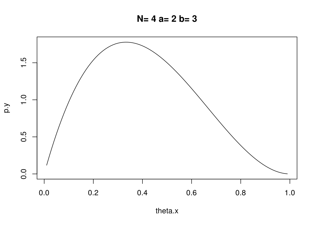
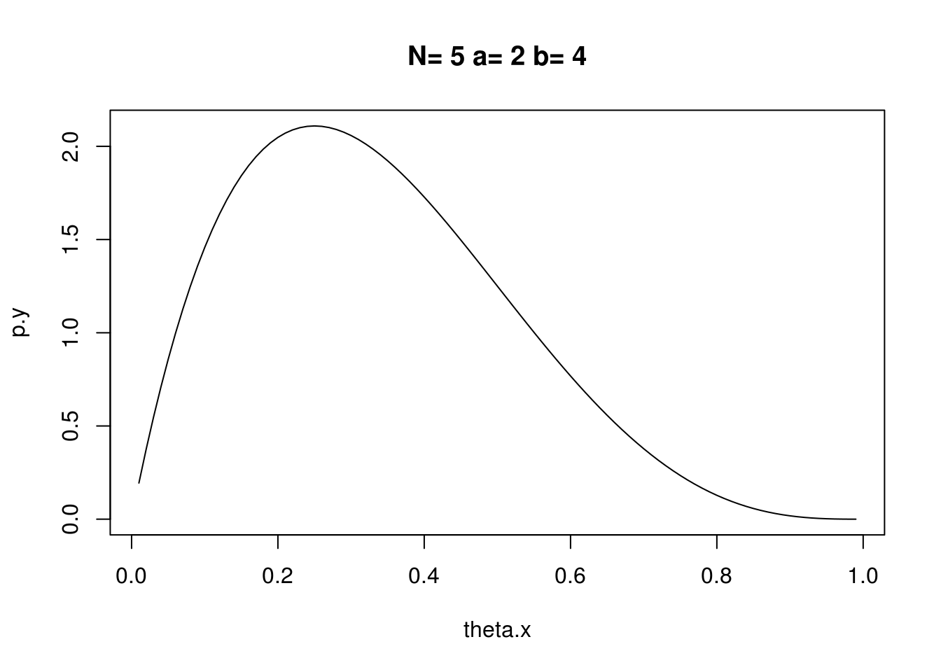
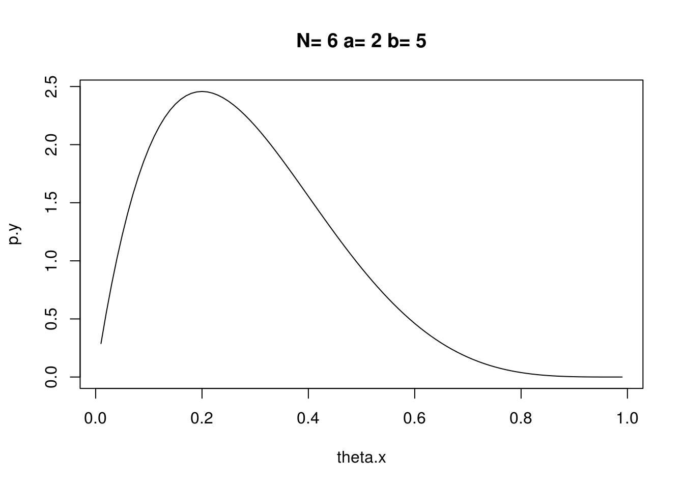
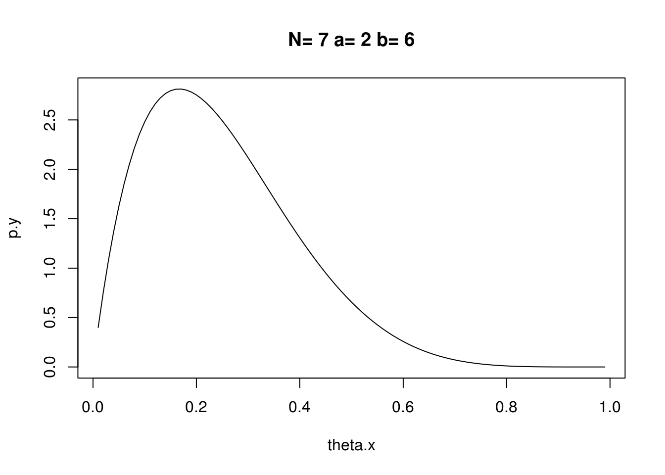
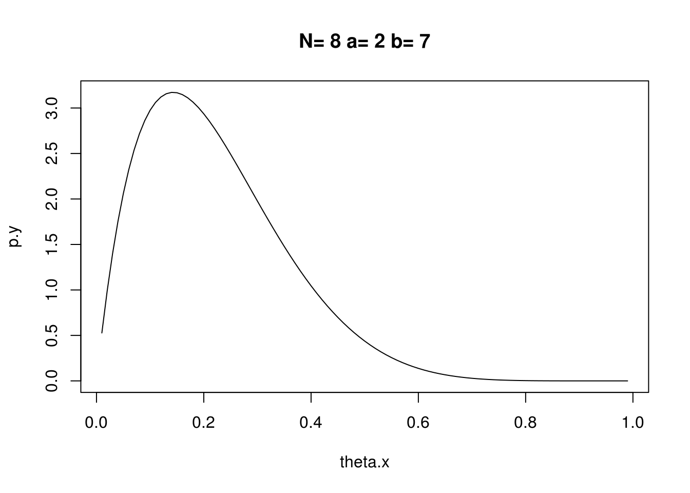
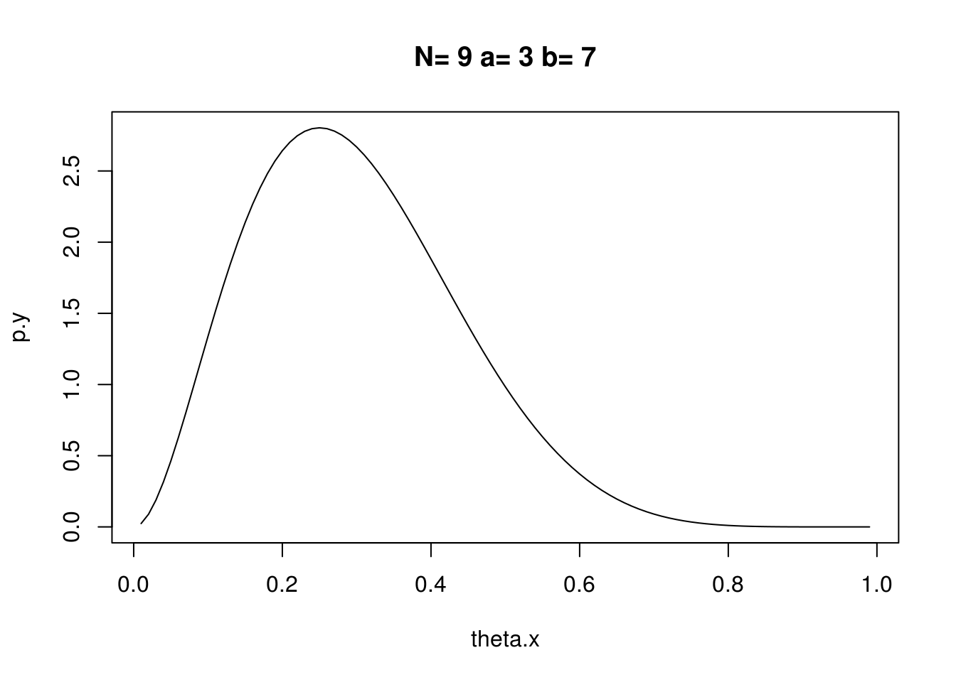
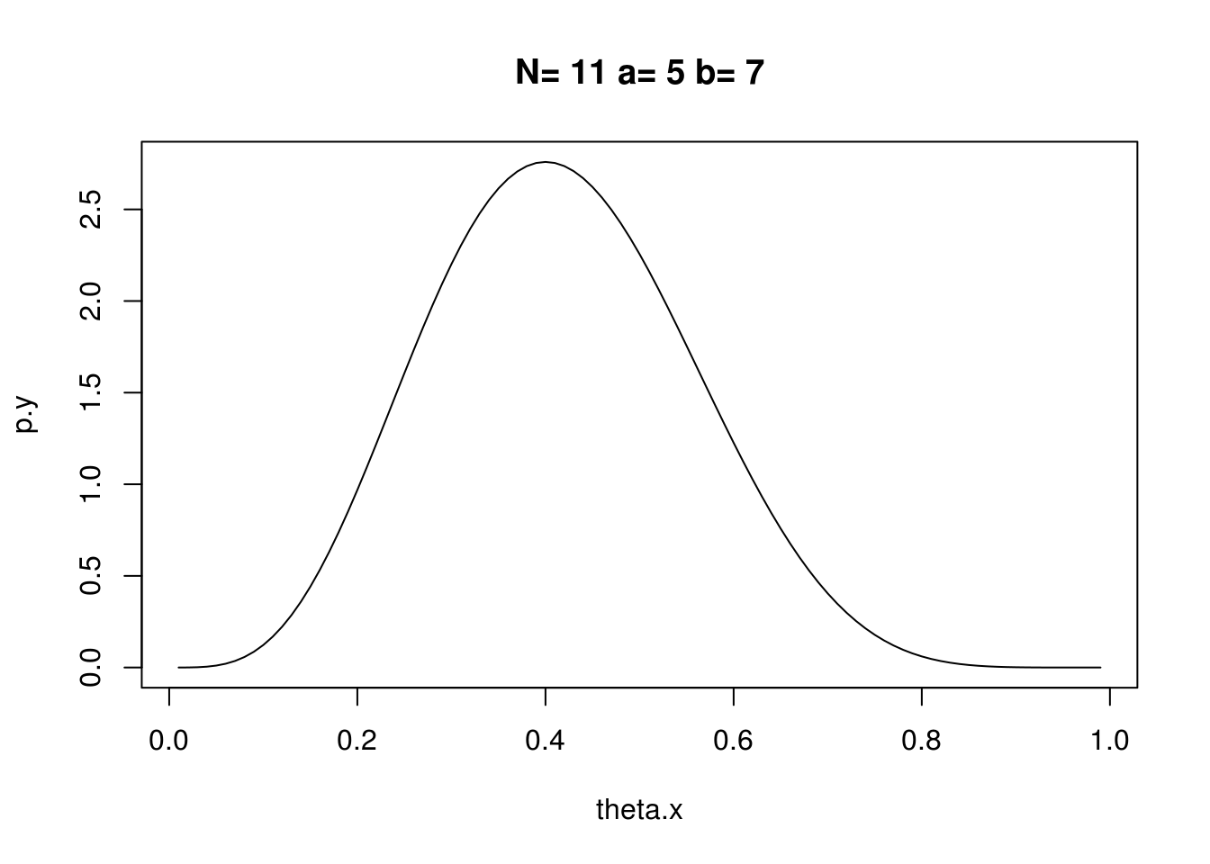
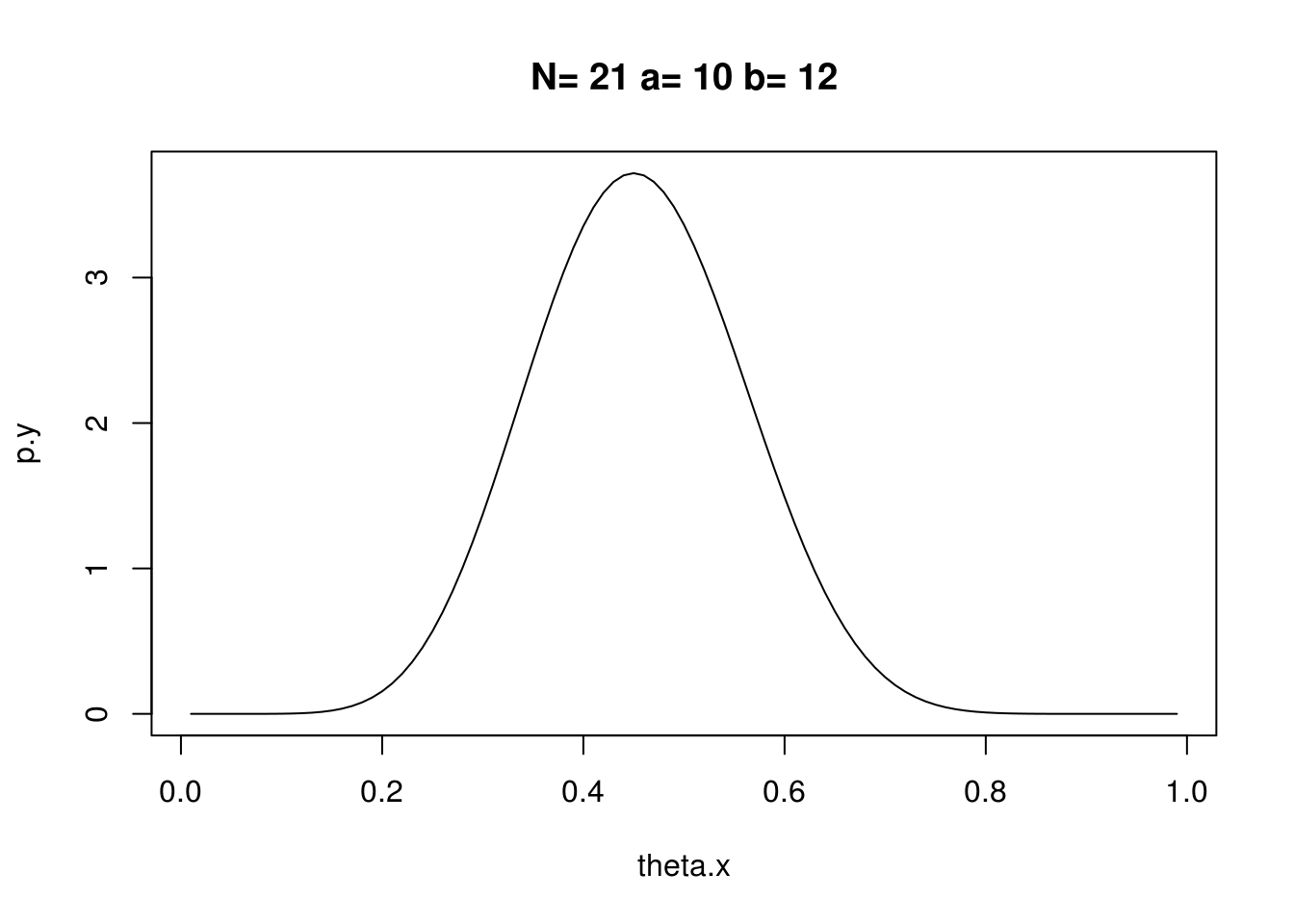
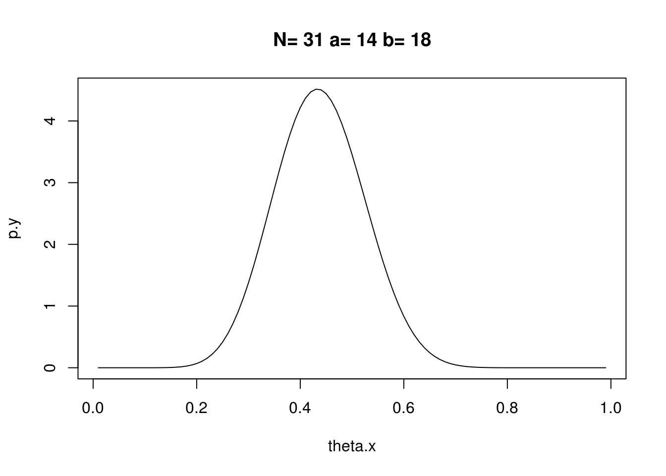
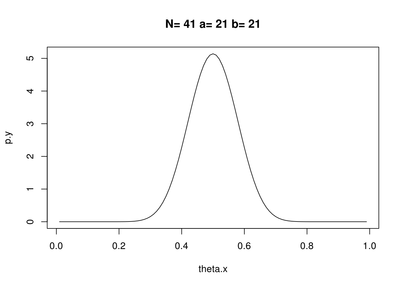
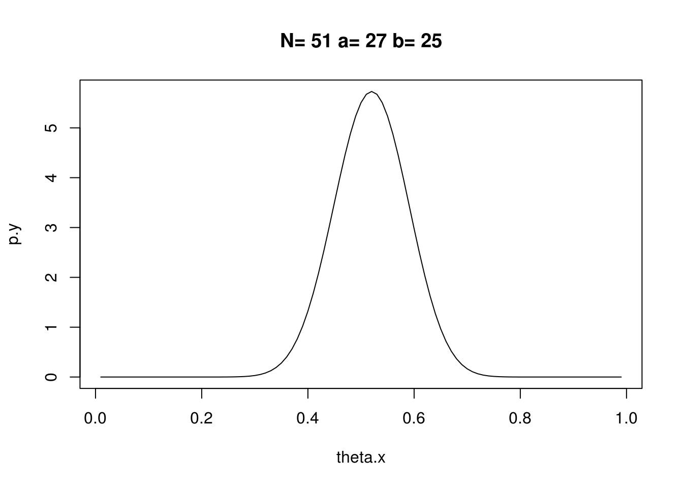
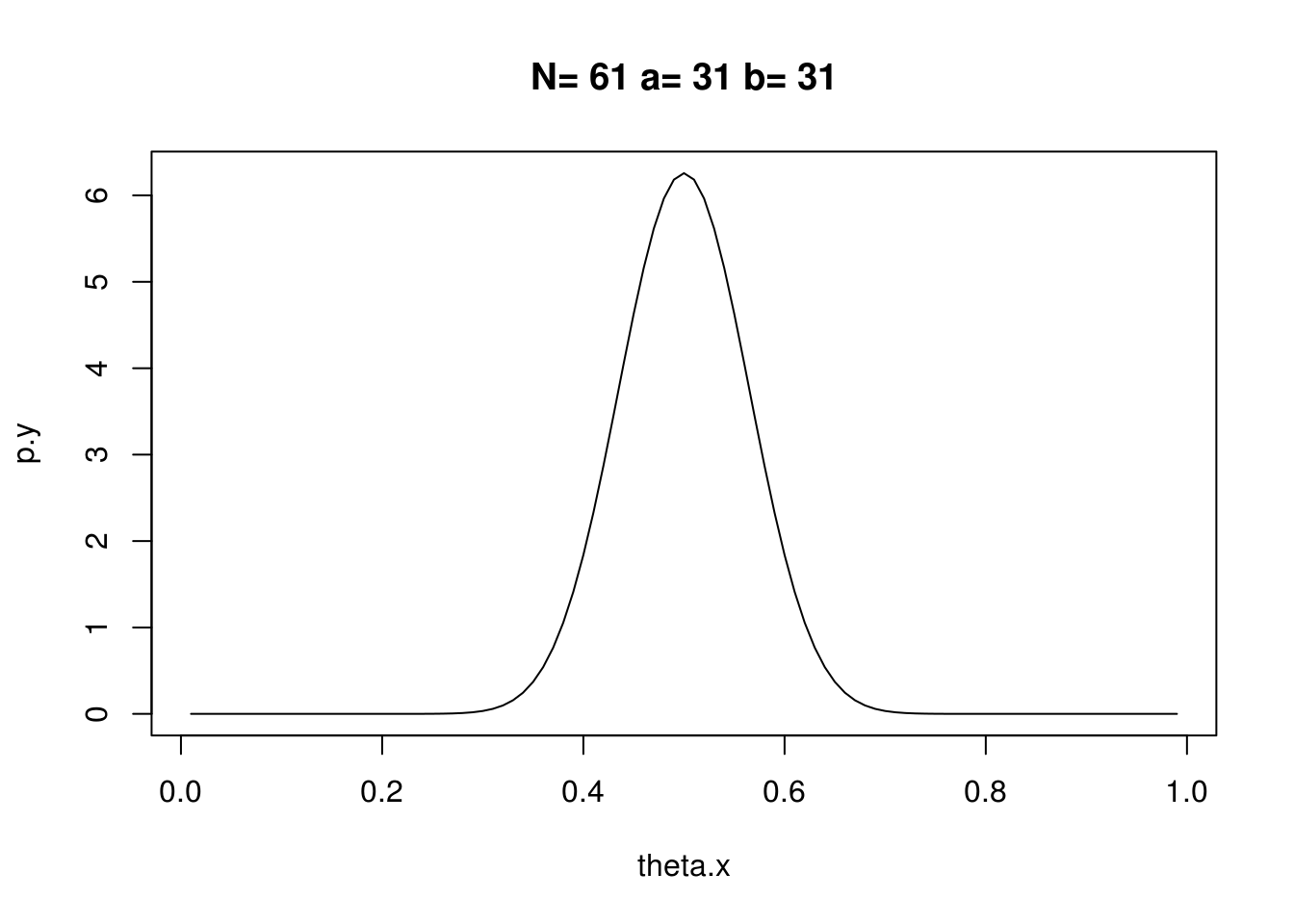
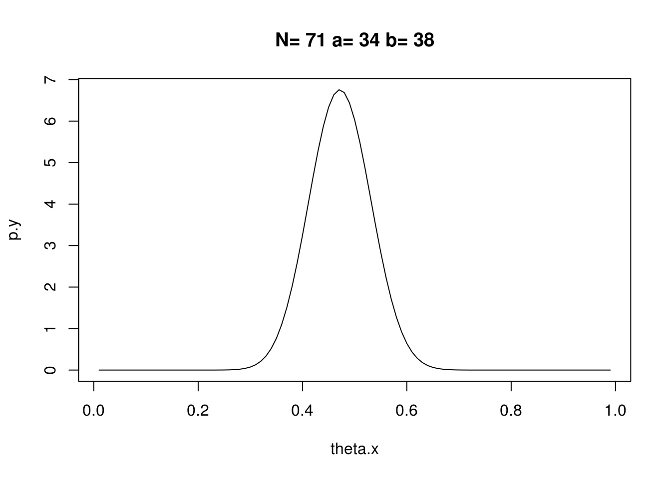
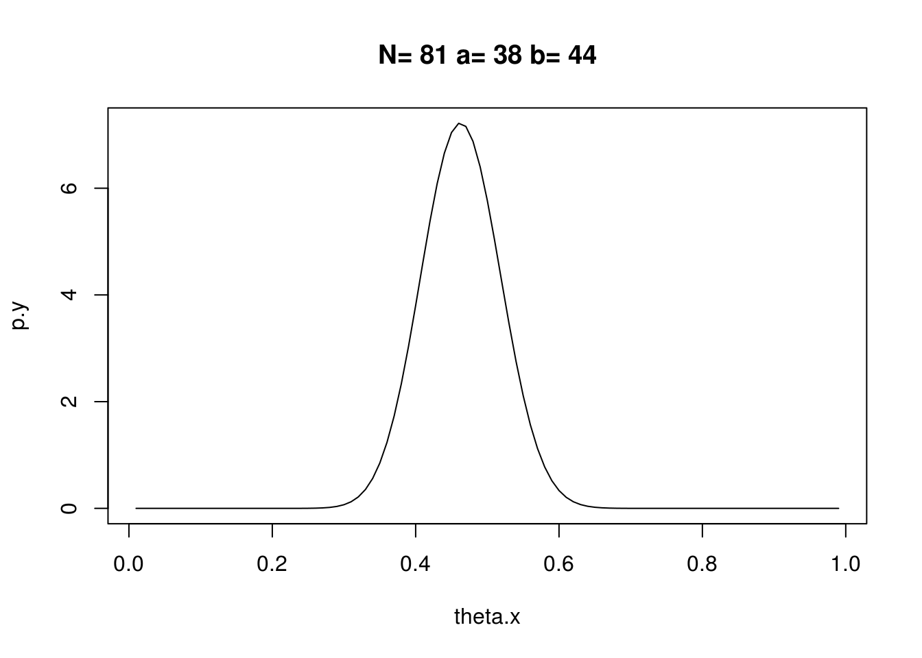
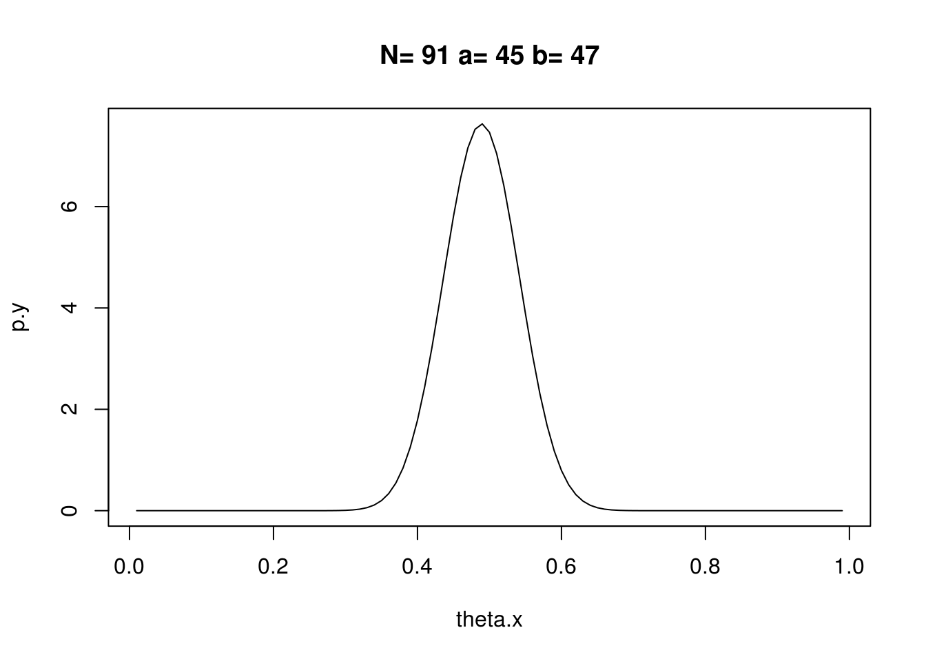
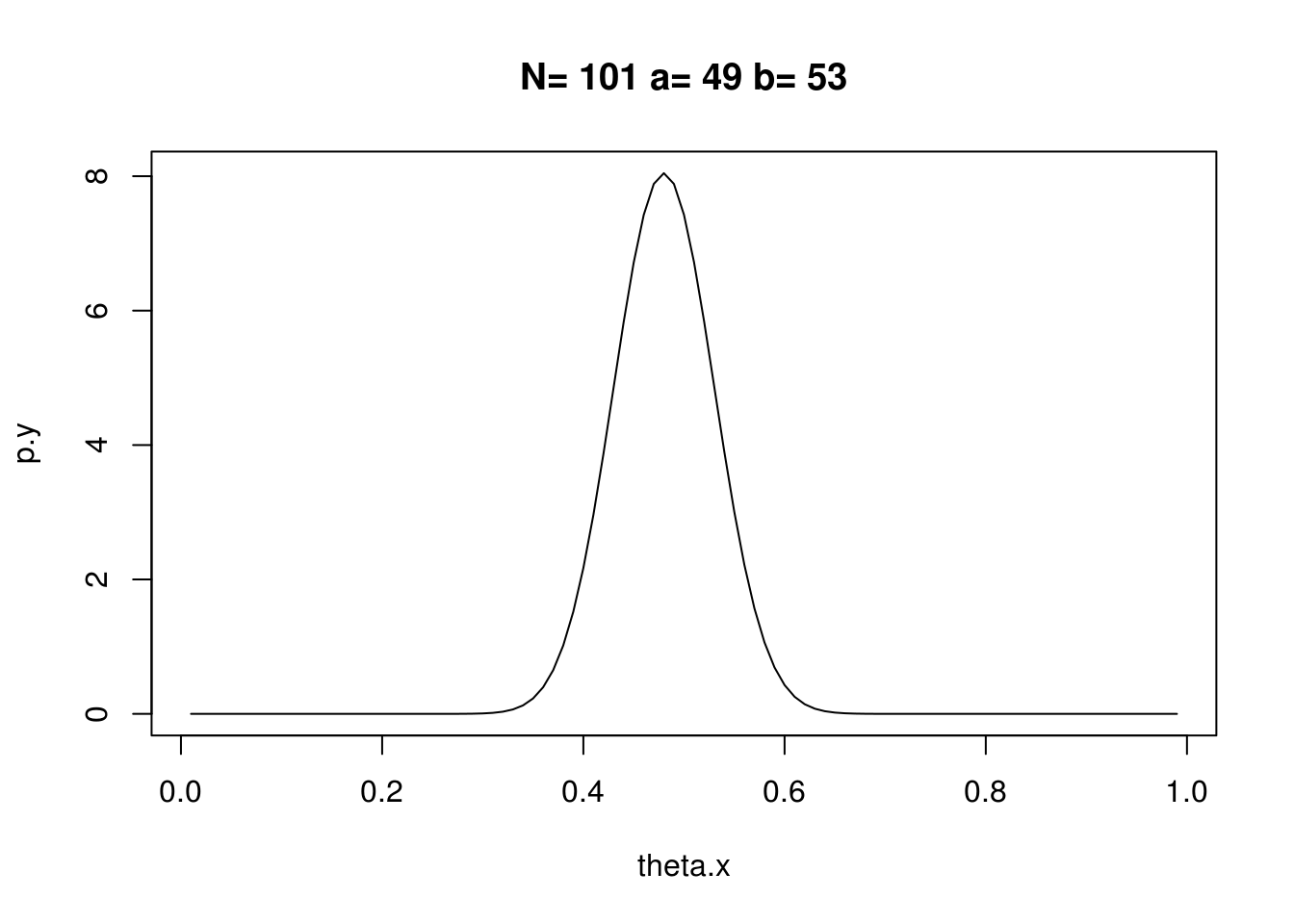
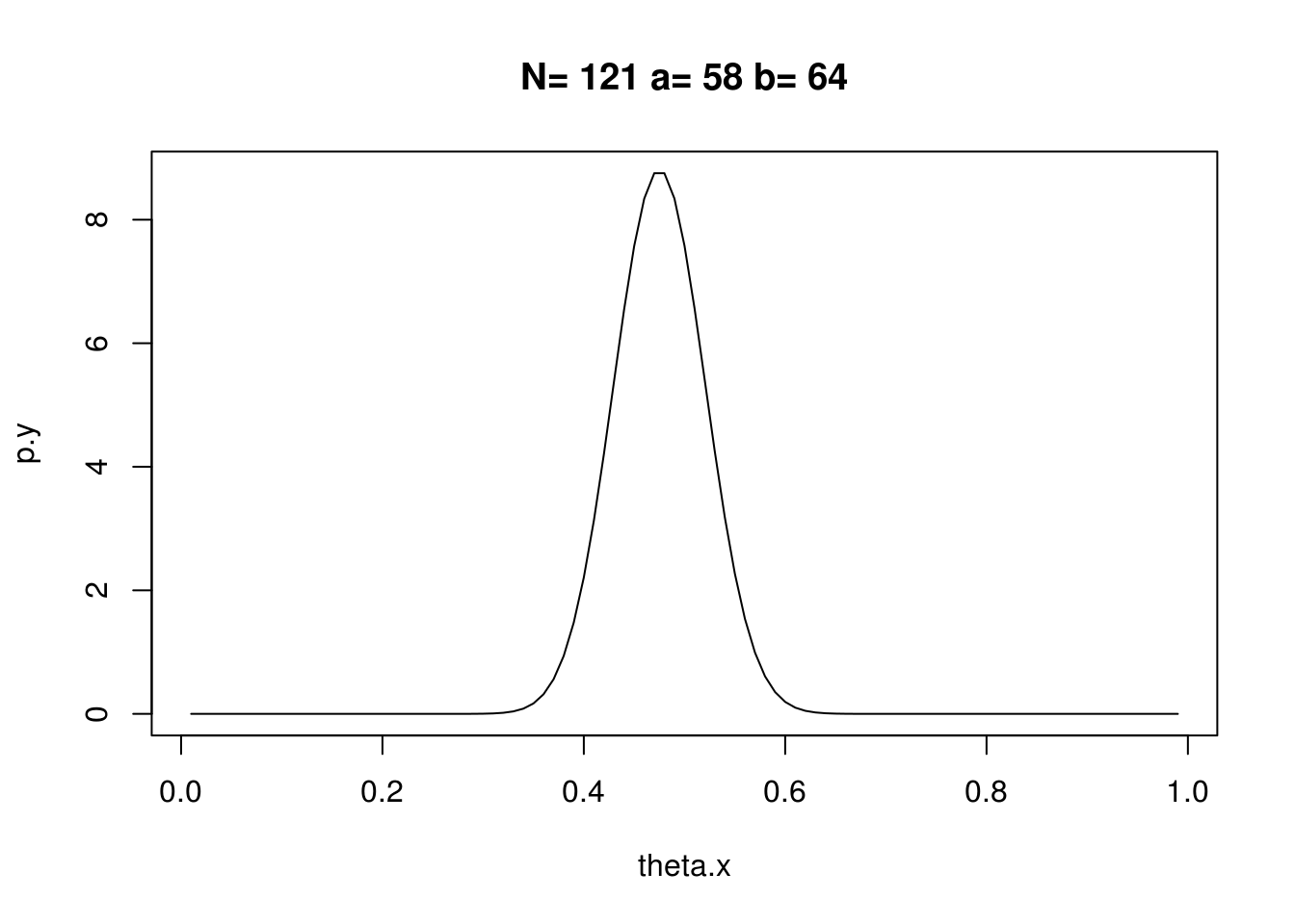
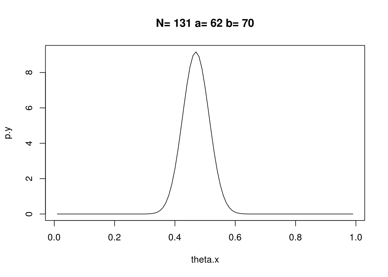
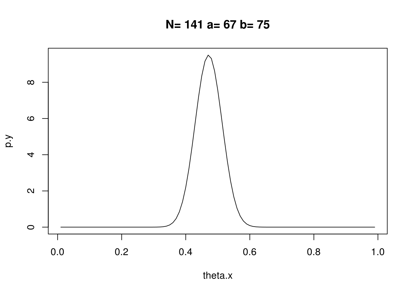
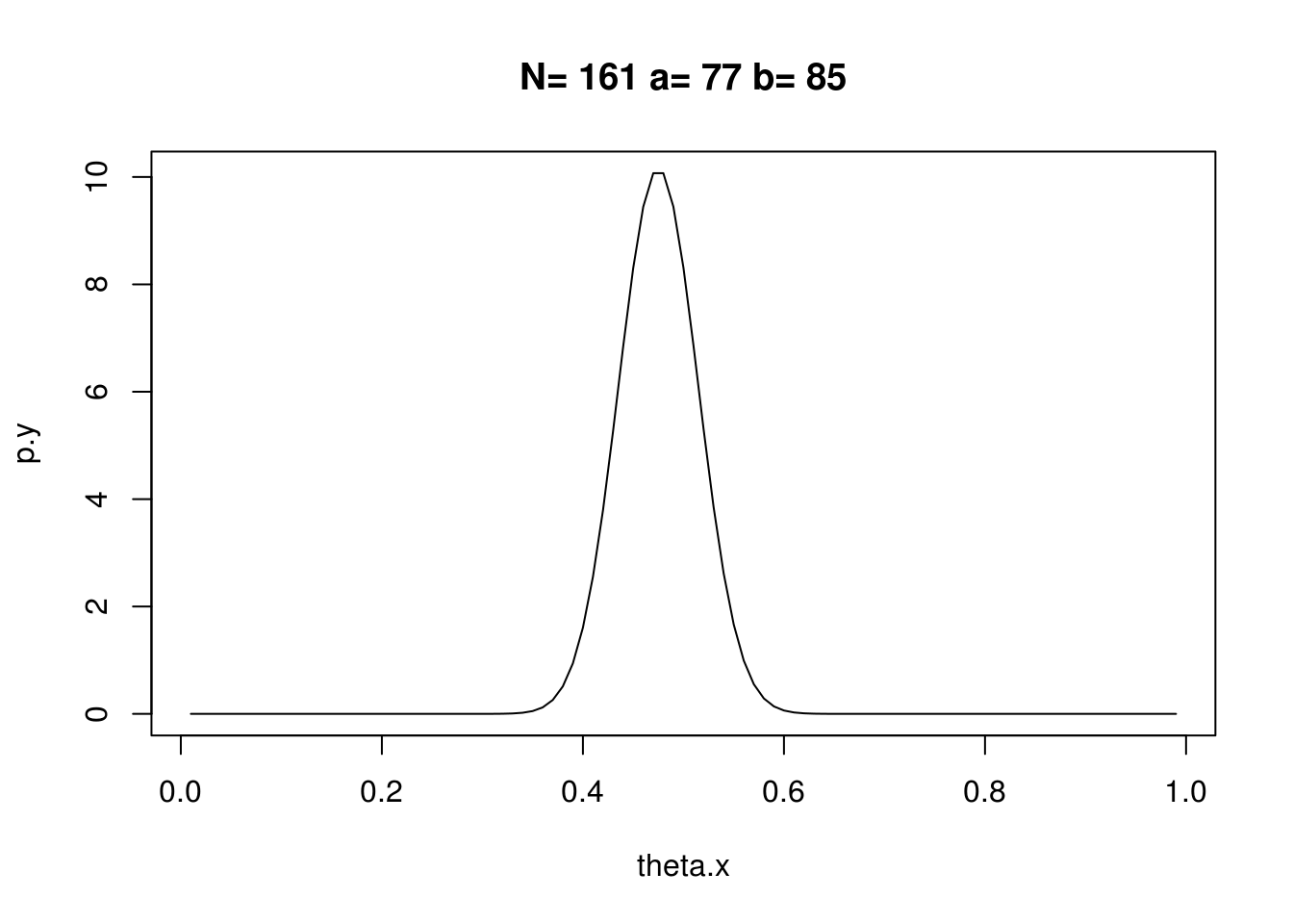
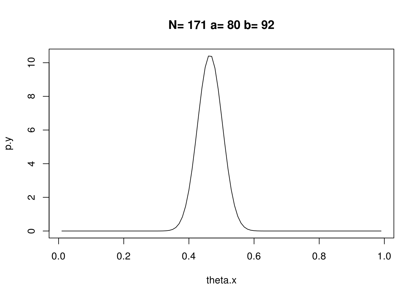
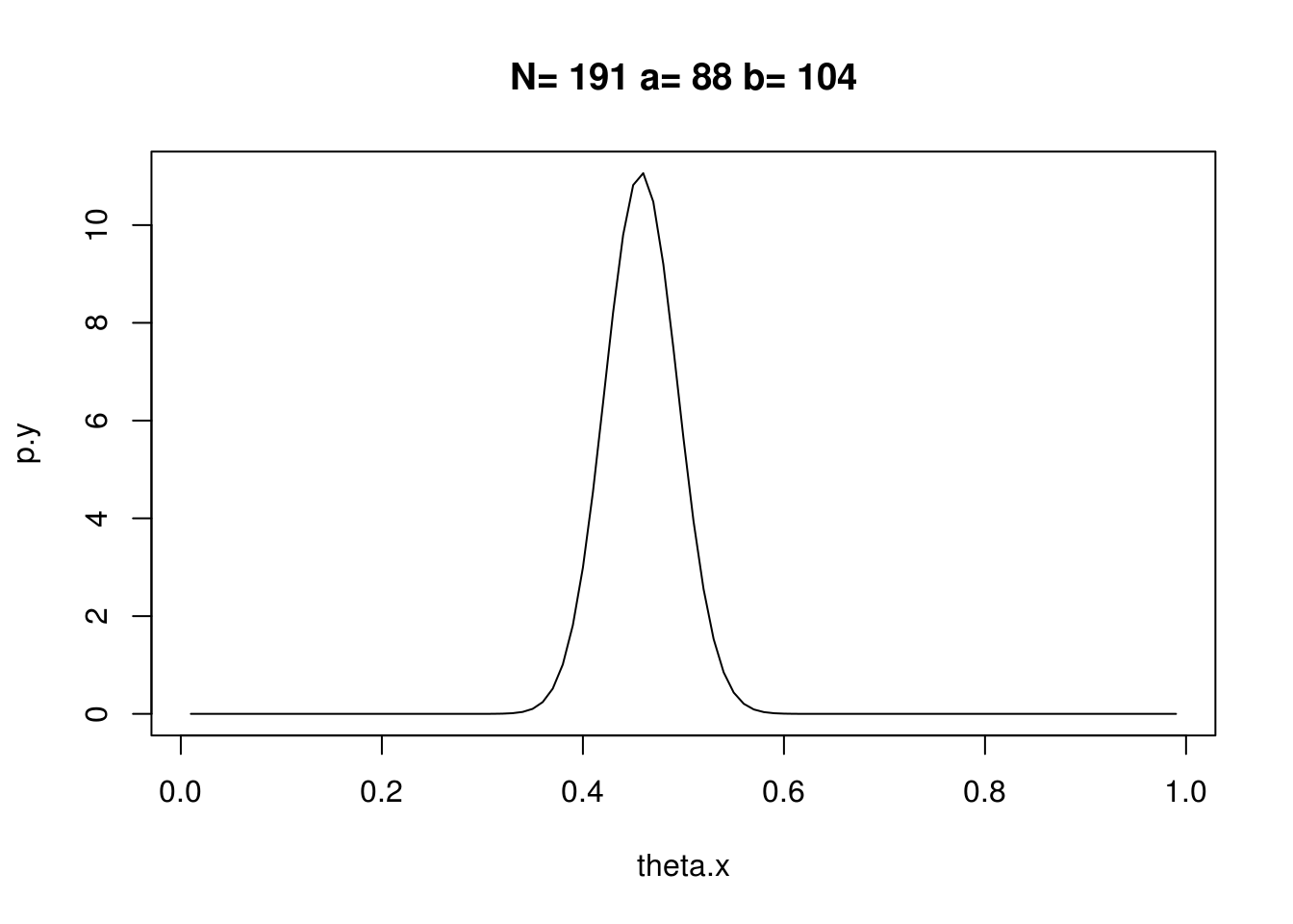
Posterior Beta Distribition evolution

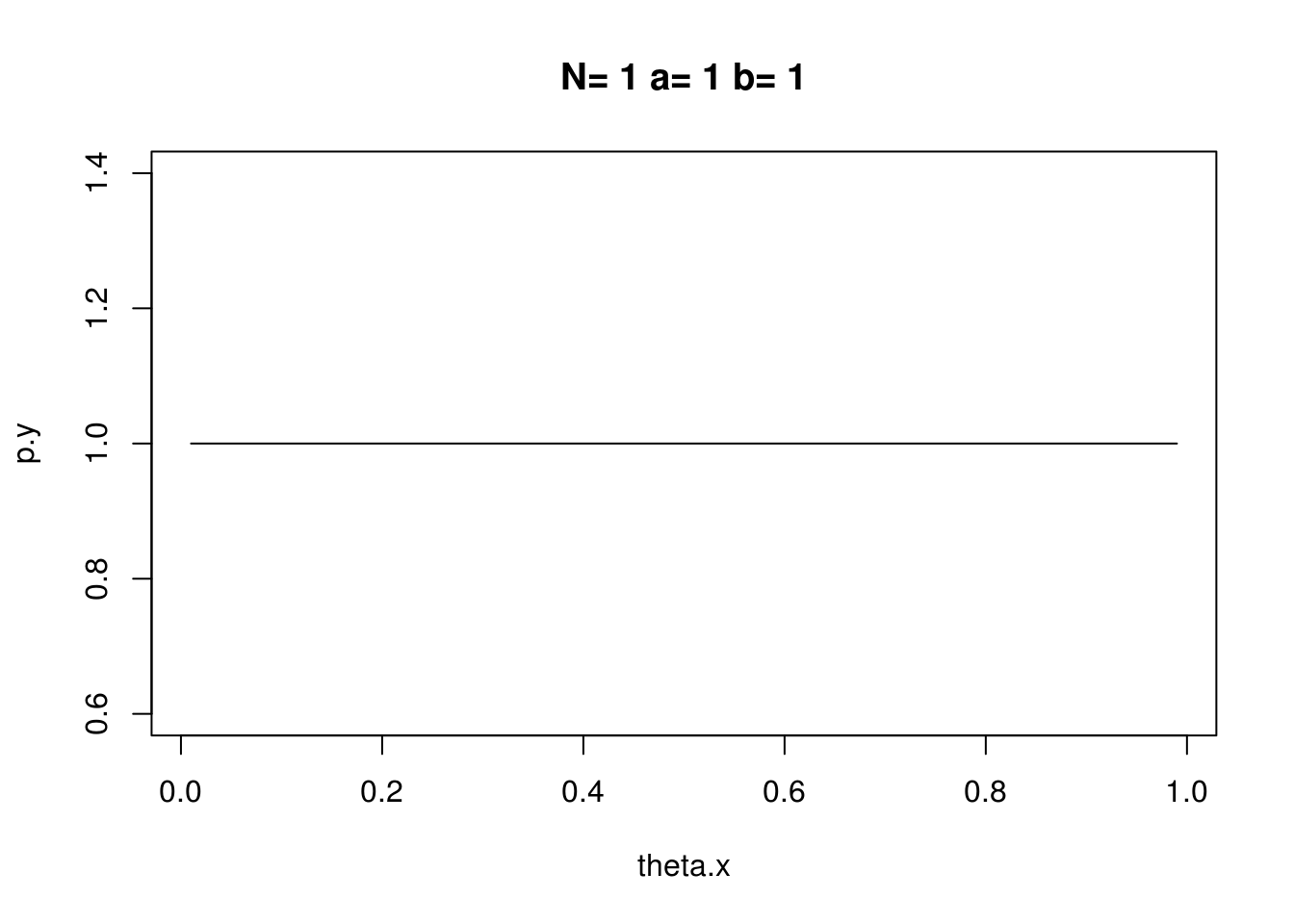
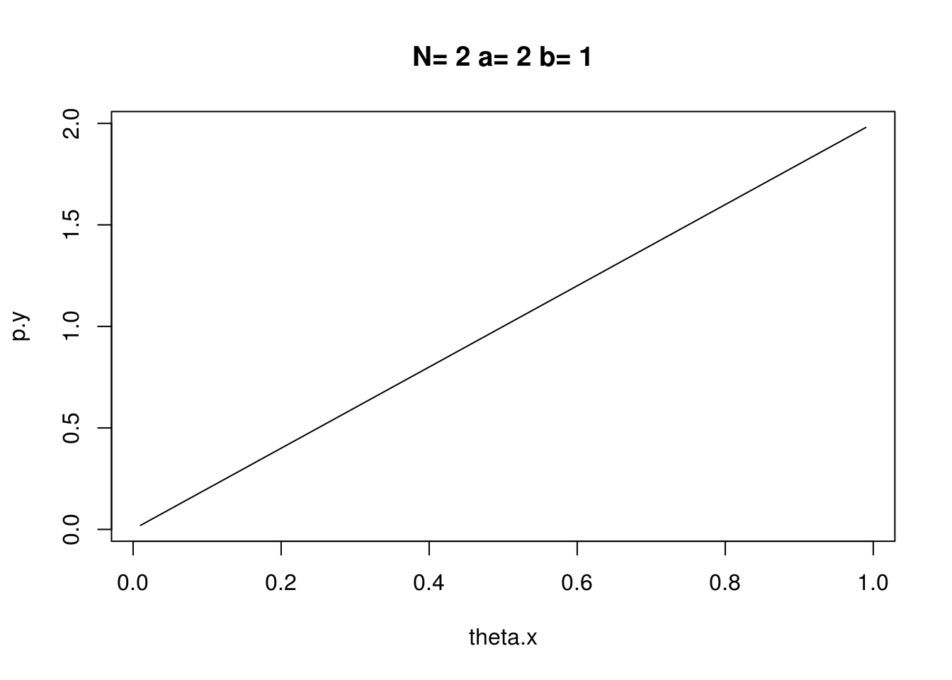
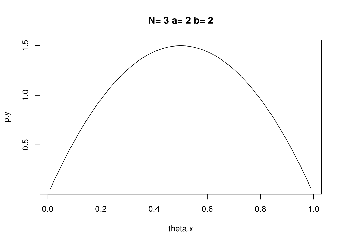
set.seed(1010101)
theta <- 0.5
N <- 200
data <- rbinom(N,1,theta)

a <- 1
b <- 1

for (i in 1:N){ # suppose patients are treated one-by-one
  if (i < 10 || i %% 10 == 1 ) {
    theta.x <- seq(0.01, .99, 0.01)
    p.y <- dbeta(theta.x,a,b)
    plot(theta.x,p.y,main = paste("N=",i,"a=",a,"b=",b),type="l")
  }
  if (data[i]==1){ # if the i-th is cured by the treatment
    # basically add 1 to a for X===1
    a <- a + 1
  } else { # if the i-th is NOT cured by the treatment
    # basically add 1 to b for X===0
    b <- b + 1
  }
  # probability of theta>1/2 based on the posterior distribution
  Ptheta <- 1 - pbeta(0.5,a,b)
}

#Posterior # Distribition # evolution

Simple Example on a Decision Rules, Admissibility, etc

We start with \(\theta>0\) and \(E[X|\theta]=\theta\) and \(Var[X|\theta]=\theta^2\)

We have a class of decision rules that are \(S=\{\delta_c(X)=cX, 0 < c < 1\}\)

and we’re give the standard squared loss funciton \(L(\theta,a) = (\theta - a)^2\)

To find a decision rule in \(S\) that is admissible means finding a decision rule \(\delta_{c}\) for there exists no other decision rule that is R-better than \(\delta_{c}\)

We can find such a decision rule by finding \(\delta_{c}\) for which the Risk is the minimum possible.

We know that the Bayesian risk for a decsion rule is defined by \(R(\theta,a)=E[L(\theta,a)]\)

Thus if \(L(\theta,a) = (\theta - a)^2\), we can substitute that back into the risk formula and get: \(R(\theta,a)=E[(\theta - a)^2]\)

Further we know that \(a\) is of the form \(\delta_c(X)=cX\) for \(c \in (0,1)\) and if we also plug that in we get \(R(\theta,\delta_{c})=E[(\theta - cX)^2]\)

so we can derive

\begin{align} R(\theta,\delta_{c})=E[(\theta - cX)^2]\\ =E[\theta^2 -2c\theta X +(cX)^2]\\ =\theta^2 - 2c\theta E[X] +c^2E[X^2] \end{align}

Now we can use the identity that \(Var[\zeta] = E[\zeta^2] - E[\zeta]^2\), which if we re-arrange, we get \(E[\zeta^2] = Var[\zeta] + E[\zeta]^2\).

Now let us set \(\zeta=\theta -cX\) and put that in our re-arranged identity and we get (Note: \(Var(X+c)=Var(X)\), and where \(Var(cX)=c^2Var(X)\) where c is a constant):

\begin{align} \require{cancel} E[\zeta^2] = Var[\zeta] + E[\zeta]^2 \\ E[(\theta -cX)^2] = Var[\theta -cX] + E[\theta -cX]^2 \\ E[\theta^2-2cX\theta +c^2X^2] = c^2Var[X] + (E[\theta] -cE[X])^2 \\ E[\theta^2]-2c\theta E[X]+c^2E[X^2] = c^2Var[X] + (\theta -cE[X])^2 \\ \theta^2-2c\theta E[X]+c^2E[X^2] = c^2Var[X] + \theta^2 -2c\theta E[X] +c^2E[X]^2 \\ \cancel{\theta^2} \bcancel{-2c\theta E[X]}+c^2E[X^2] = c^2Var[X] + \cancel{\theta^2} \bcancel{-2c\theta E[X]} +c^2E[X]^2 \\ \xcancel{c^2}E[X^2] = \xcancel{c^2}Var[X] +\xcancel{c^2}E[X]^2 \\ E[X^2] = Var[X] + E[X]^2 \end{align}

next let us substitute it back into our previous result:

\begin{align} R(\theta,\delta_{c})=\theta^2 - 2c\theta E[X] +c^2E[X^2] \\ =\theta^2 - 2c\theta E[X] + c^2(Var[X] + E[X]^2) \\ =\theta^2 - 2c\theta E[X] + c^2Var[X] + c^2E[X]^2 \end{align}

Now we plug back \(E[X|\theta]=\theta\) and \(Var[X|\theta]=\theta^2\) into the previous result:

\begin{align} R(\theta,\delta_{c})=\theta^2 - 2c\theta E[X] + c^2Var[X] + c^2E[X]^2 \\ =\theta^2 - 2c\theta \cdot \theta + c^2\theta^2 + c^2(\theta)^2 \\ =\theta^2 - 2c\theta^2 + 2c^2\theta^2 \\ =\theta^2 \end{align}
#bayesian #decision-rule